Join Quality Metric
Link to notebook. The notebook includes all the necessary code to create the data and generate the plots. Nonetheless, an iteration of this data is already contained here, under the k_justification folder.
Here we focus on developing a novel join quality measure specifically for data lakes, which combines a syntactic set overlap computation (Multiset Jaccard, MJ) and the Cardinality Proportion (K) to lightly indicate semantic relatedness:
Preparing the data
First, we define functions to compute all the necessary metrics (Multiset Jaccard, Jaccard, containment, and the cardinality proportion). This allows us to compare the basic set-overlap metrics and discern which is best (and later combine them with the cardinality proportion). We start by loading the ground truth, which is a dataframe of joins (pairs of attributes from different datasets) with the following measurements: containment (C), cardinality proportion (K), Jaccard (J) and multiset Jaccard (MJ) scores. MJ and K will be used to derive the final metric, whereas C and J will be used as baselines to test the effectiveness of MJ. Additionally, each join is assigned a type of relationship (semantic or syntactic). A join is syntactic if containment > 0.1. A join is semantic if, on top of being syntactic, the columns have a meaningful relationship (e.g., both columns represent countries). This assignment has been done manually.
Initial experiments
We conduct a series of initial experiments that showcase that Multiset Jaccard is better suited for joinability detection than both containment and Jaccard, mainly by checking how well these metrics can separate semantic from syntactic joins. This is likely due to Multiset Jaccard taking into consideration multisets, which provides an advantage in denormalized scenarios, such as data lakes, where repeated values are common. Nonetheless, the results are not good enough, so we need a way to improve them.
We start by ordering the joins in three different "rankings," one per each set overlap metric, with higher values placed at the top. Then, we separate each ranking into its four quartiles and measure the proportion of semantic and syntactic joins in each. Ideally, for quartiles 3 and 4 (representing the top 50% of joins), they should have a higher proportion of semantic joins than quartiles 1 and 2. Note that the ground truth contains more syntactic than semantic joins.
Result: Containment is clearly worse than both Jaccard metrics in developing this separation. Multiset Jaccard seems to make the distribution slightly better than Jaccard, although the evidence is small.
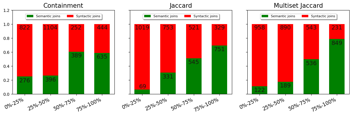
Figure 1. Comparison of semantic and syntactic join proportions across quartiles for Containment, Jaccard, and Multiset Jaccard.
Since a real user only considers the top $k$ joins, we now focus on the Precision at $k$ (P@k) metric: how many of the top $k$ joins are semantic? We set $k$ to 100, which is far more than a realistic end user would consider.
Result: We can observe that Multiset Jaccard is clearly better at placing semantic joins in the top spots. Both containment and Jaccard place syntactic joins in the first few positions, meaning the first joins given to the user would be false positives. We have a clear argument to prefer Multiset Jaccard.
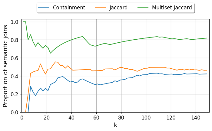
Figure 2. Precision at $k$ (P@k) for Containment, Jaccard, and Multiset Jaccard, showing performance for top joins.
Relevance of K
We move to testing the relevance of the cardinality proportion (K) for join detection. We observe that the proportion of K for syntactic and semantic joins varies considerably, which indicates that K can be used as a complimentary and lightweight assessment of join quality in the context of data lakes.
This variation can be seen by comparing the distribution of K for semantic and syntactic joins.
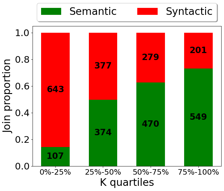
Figure 3. Distribution comparison of the Cardinality Proportion (K) for semantic and syntactic joins.
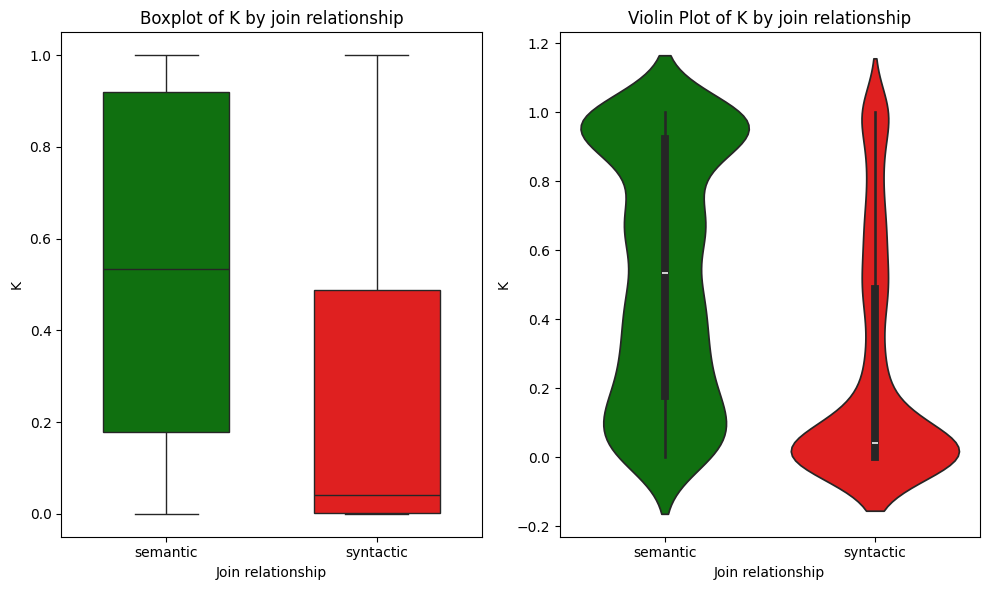
Figure 4. Violin plot showing the distribution of the Cardinality Proportion (K) for different join types.
Multiclass metric
Once we have decided on the use of MJ and K, we create a conjoined metric that takes both measurements into account. By plotting the scores for MJ and K obtained by the ground truth, we can observe a positive correlation between the values of the metrics and the semantic category of the joins: the higher the values of MJ and K, the more likely a join is semantic.
Hence, we define a discrete multiclass metric that maps the ground truth instances onto four (by default, but there might be many levels) quality categories, ensuring that the "higher" buckets contain a greater proportion of semantic joins compared to syntactic joins. This is not meant to define 100% accurate thresholds, but rather to capture general trends. The selected function is arbitrary, as there is an infinite amount of functions to try; our proposal is a reasonable choice among many. We plot the result of applying such function over our ground truth.
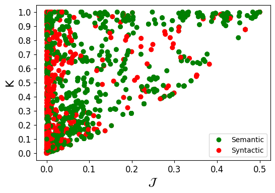
Figure 5. Scatter plot of Multiset Jaccard (MJ) versus Cardinality Proportion (K) categorized by binary join type.
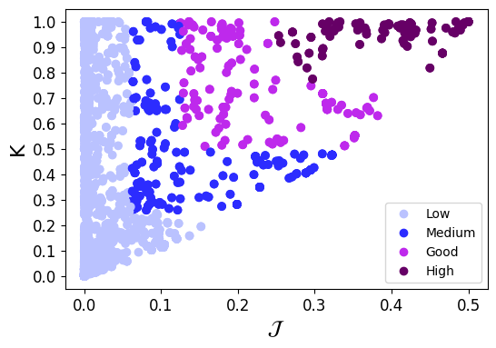
Figure 6. Scatter plot of Multiset Jaccard (MJ) versus Cardinality Proportion (K) using the four quality multiclass metric.
Finally, we transform the multi-class metric to a continuous one to allow for rankings. To do so, we fit the discrete metric to a continuous function by computing the Wasserstein distance between the discrete function and continuous functions generated from Gaussian distributions with a series of fixed parameters. The final continuous function is the one that minimized the Wasserstein distance for both K and MJ. We also showcase that $L = 4$ (four buckets) is the value that minimizes the distances, hence it is the value selected for the final function.
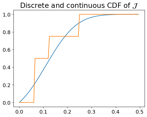
Figure 7. Continuous fitting of the discrete metric for the Cardinality Proportion (K).
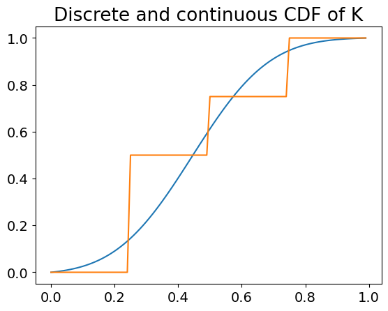
Figure 8. Continuous fitting of the discrete metric for Multiset Jaccard (MJ).
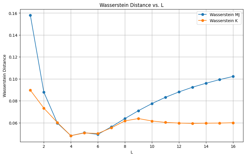
Figure 9. Wasserstein distance as a function of the number of classes $L$.
Strictness
Finally, to facilitate reproducibility, we add a strictness measurement to the metric, which can alter its behavior to be more restrictive. The higher the strictness, the more restrictive the scoring will be. That is, a higher strictness value implies that higher scores of MJ and K are necessary to achieve a high join quality score. We define three levels: relaxed, balanced (which is the one we build the final model with), and strict. As we want to provide a single model to prevent cumbersome configuration for the user, we build the final model with the balanced strictness value.
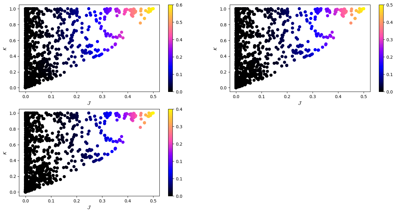
Figure 10. Comparison of the final metric's performance under different strictness levels (relaxed, balanced, strict).
last updated: 2026/01/07